How Predictable Death by COVID-19 Incidence?

I downloaded from the European Centre for Disease Prevention and Control website the daily database constituting the number of new cases reported and death worldwide due to COVID-19. The database had 13,623 daily records from December 31, 2019 to April 28, 2020. I summed records by country and filtered the number of incidences avoiding outliers using a statistical formula.  The filtered record shows a list of 136 countries that had an incidence in 314,099 persons, of which 7,866 persons died. It shows that 2.5 percent of infected people had already died and there is a possibility of other deaths too, which the time will tell. Israel had a maximum of 15,598 incidences, and the British Virgin Islands had a minimum of 6 incidences. Algeria had a maximum of 437 deaths and 13 countries each had one death.

Then, I calculated the Pearson correlation coefficient between the number of incidence and deaths for the filtered records.  The purpose of removing outliers was because the Pearson correlation coefficient works when the datasets are close to normal distribution. The analysis shows a correlation coefficient of 0.677 which was significantly different from zero (p=0.01). This suggests that there is a moderate chance of death if one is infected with COVID-19. A regression analysis was also conducted to predict death based on incidence, which gives an R square value of 0.459 indicating that nearly half the variation in the number of deaths is explained by the model. A significant coefficient indicates that the number of incidences significantly contributes to the model. For every 1000 incidences 18 deaths are likely.

Graphics Visualizing Target Population

Graphics is an important form to visualize one data from others. This technique is useful to visualize the target population for any purpose. For example, I referred to Nepal’s population census 2011 data to get population values to visualize the number of male household heads from urban areas of Nepal belonging to the age group of 50 years and above. I used four criteria to filter and get target population data – male, age group, administrative setting (urban), and position or role in a household (household head).

An outermost blue circle shows the total population of Nepal, which is 26,494,504. It is followed by a red circle showing the male population which is 49 percent of the total population. An inner third yellow circle shows the male population aged 50 years and above, which is 15 percent of the total male population. An inner dark ash-colored circle shows the urban male population aged 50 years and above, which is 15 percent of the total males aged 50 years and above. Lastly, an innermost green circle shows the number of urban male household heads aged 50 years and above, which is 81 percent of total urban males aged 50 years and above and 1.9 percent of the total male population in Nepal.

These data are visualized in both stacked Venn and horizontal hierarchical diagrams in Figures 1 and 2 respectively.

Figure 1: Target population of urban male household heads aged 50 years and above shown in a stacked Venn diagram

Figure 2: Target population of urban male household heads aged 50 years and above shown in a horizontally hierarchical diagram

In a nutshell, visualizing filtered data in different diagrammatic forms is a cool way.

Level of Confidence Increases with Sample Size: An Example of One Sample Proportion, Statistical Note 47

Level of confidence increases with an increase in sample size for one sample proportion. This note tries to exemplify this fact by using the process and data discussed in my statistical note 43 and 44 respectively.

For example, an expert is interested in knowing the proportion of non-smokers from the randomly sampled respondents (following randomization, the first rule of sample proportion). An expert assumes that half of adult population are smokers. An expert administers a question to the randomly adults – Are you a smoker? The respondents answer to one of two categories of response – Yes or No.

An expert tries with a sample size of 100 adults and finds that 55 are non-smokers and remaining 45 are smokers (following normality that non-/smokers need to be at least 10, second rule of sample proportion). An expert then retains the same sample proportion of smokers and hypothetically increases the sample size by 100 to 500. An expert assumes to follow independence in sampling without replacement that the population size is more than 10 times of sample size, third rule of sample proportion.

An expert estimates how confident he is in deciding that non-smokers statistically outnumber the smokers with the increase in sample size. An expert uses the following formula to calculate the minimum number of non-smokers from the given sample size to outnumber the smokers:

 z=(p^-p)/√(pq/n)

  where ,

z=Test statistic, standard normal variate, with a value of 1.96 at 95% level of confidence

p^=Sample proportion of non-smokers

p=Population proportion of non-smokers, equal to 0.50

q= Population proportion of smokers, equal to 0.50

n=Sample size

Table 1: Sample size with Same Sample Proportion of Non-Smokers and Level of Confidence to Conclude Non-Smokers Outnumber Smokers

An expert is 84 percent confident in deciding that the sample non-smoker proportion of 0.55 among 100 respondents statistically outnumbers the sample smoker proportion of 0.45. Usual threshold is that decisions are made at 95 percent level of confidence. Gradually, an expert increases sample size by 100 and finds that for a sample of 300 respondents or more an expert is more than 95 percent confident in deciding that the sample proportion of non-smokers equal to 0.55 is statistically higher than the sample proportion of smokers equal to 0.45. It proves that the level of confidence increases as sample size increases for one sample proportion.

Conditional and Joint Probabilities from an Exemplary Survey Dataset, Statistical Note 46

Understanding the concepts of joint and conditional probabilities and developing the skill to apply the concepts to calculate from the given dataset is important in the real time.

An exemplary survey dataset constitutes one hundred records of randomly sampled respondents categorized by smoking habit (smokers or non-smokers) and food habit (vegetarians or non-vegetarians). A part of the dataset in value label view of SPSS is shown in Table 1. Calculate the probability that a randomly sample respondent is a non-smokers is a non-vegetarian.

Table 1: Part of a dataset with smoking and food habits

Concept

Calculating the probability of a "AND" compound event that a randomly selected respondent is a smoker who is a vegetarian also includes calculating the probabilities of other events. Several concepts are introduced while answering this question.

This example has two discrete random variables or categorical variables each with two mutually exclusive categories of response. One categorical variable is the smoking habit of a randomly sampled respondent which has two categories of response: smoker (S) or non-smoker (NS). Another categorical variable is the food habit which also has two mutually exclusive categories: vegetarian (V) and non-vegetarian (NV).

Simple or marginal probability: Let ‘S’ be a random event that a randomly sampled respondent is a smoker. The probability of randomly sampled smoker, represented by P(S) is the total number of smokers divided by total number of respondents. It is also referred to as the relative frequency. Similarly, P(NS), P(V) and P(NV) are calculated.

Conditional probability: Let V/S be a simple event that a participant is a vegetarian among the smokers. The conditional probability of vegetarians among smokers symbolized by P(V/S) is total number of vegetarians among smokers divided by total number of smokers. Here the occurrence of the event of vegetarian smoker is dependent on the event of occurrence of smokers.

Joint Probability: Let ‘S intersection V’,  ‘S∩V’ or ‘S and V’ is a "AND" compound event that a respondent is a smoker and a vegetarian. Here, the multiplication rule of two dependent events is applied. The joint probability of two dependent events is the product of a marginal probability and the conditional probability. In this case, the joint probability of a smoker who is a vegetarian indicated by P(S intersection V), P(S∩V) or P(S and V) in which both events of smoker and vegetarian among all smokers occur is the product of P(S) and P(V/S). Likewise, P(NV/S), P(V/NS), P(NV/NS), P(NS∩V), P(S∩NV) and P(NS∩NV) are calculated.

Calculation

A contingency or cross table from the given survey dataset can be generated either in SPSS or Excel package upon the availability of the software.  In SPSS, using the function ‘Crosstabs’ in Descriptive Statistics’ group of ‘Analyze’ tab, one can get the cross table as in Table 2. In Excel, ‘Pivot Table’ function in the ‘Tables’ group in ‘Insert’ tab can be used to generate cross table like this.

Table 2: Cross table of smoking habit and food habit

Table 2 constituting four cells and totals to presents the frequencies, row percent (% within SMOKE), column percent (% within VEG) and percent of total respondents. Now, the concepts discussed above are applied to calculate probabilities.

Simple or Marginal Probability: Table summarizes that 25 out of 100 respondents are smokers so that P(S) is equal to 0.25, which is 25 percent in percentage term as shown by ‘% of Total’. P(NS) is 0.75 or 75 percent in percentage term. Likewise, P(V) is 0.25 or 25 percent in percentage term and P(NV) is 0.75 or 75 percent in percentage term.

Conditional Probability: P(V/S) is calculated looking at the first cell of the table. Eight out of 25 smokers are vegetarians so that P(V/S) is equal to eight divided by 25 equal to 0.32, which is equal to the row percent (% within SMOKE) of 32% in percentage terms. Similarly, other conditional probabilities are calculated as P(NV/S)=0.68, P(V/NS)=0.227, P(NV/NS)=0.773.

Joint probability: P(S∩V) is the product of P(S) and P(V/S), equal to the product of (25 by 100 ) and (eight by 25), equal to 0.08 or 8 percent in percentage term. This is equal to ‘% of Total’ in the first cell of Table 2.

Upon filling manually the probability values in yellow highlights of Table 2, the table looks as Table 3. The joint probability for each cell is equal to percent of total value in percentage term.

Table 3: Cross table of smoking habit and food habit with probabilities manual added

It is hoped that such a simple example will help create curiosity among the readers as to applying the concept in the real time data.

Simple Probability Calculation from an Exemplary Survey Dataset, Statistical Note 45

Understanding the concept of simple or marginal probability and developing the skill to apply the concept to calculate from the given dataset is important in the real time.

An exemplary survey dataset constitutes one hundred records of randomly sampled respondents categorized as smokers or non-smokers. A part of the dataset in value label view of SPSS is shown in Table 1. Calculate the probability that a randomly sample respondent is a non-smokers.


Table 1: Part of dataset of smokers and non-smokers

Concept 

Simple or marginal probability of an event is the total number of favorable cases divided by total number of cases. Let ‘S’ be a simple event that a participant is a smoker and the simple or the marginal probability of ‘S’ represented by P(S) is the total number of smokers divided by total number of respondents. It is also referred to as the relative frequency.

Calculation 

The survey dataset can be summarized either in SPSS or Excel package upon the availability of the software.  In SPSS, using the function ‘Frequencies’ in Descriptive Statistics’ group of ‘Analyze’ tab, one can get the frequency table as in Table 2.
 

Table 2: Frequency table of smokers and non-smokers

In Excel, ‘Descriptive Statistics’ function in the ‘Data Analysis’ Add-In program can be used to generate frequency table.

The percent or valid percent column shows that 20 percent of respondents are non-smokers. It means that 20 out of 100 respondents are non-smokers.   Thus, the simple or marginal probability that a randomly sampled respondent is a non-smokers is calculated as 20 divided by 100 equal to 0.20. Similarly, the simple or marginal probability of smokers can be calculated to be 0.80.
 I hope this simple example will help create curiosity among the readers as to applying the concept in the real time data.

Same Sample Proportion with Different Sample Sizes for Chi-Squared Test for Goodness of Fit, Statistical Note 44

The level of confidence for statistical significance varies with the variation in the sample size of the same sample proportion.

For example, an expert is interested in knowing the proportion of smokers from the randomly selected sampled respondents. An expert assumes that half of adult population are smokers. An expert administers a question to the adults – Are you a smoker? The respondents respond to one of two categories of response – Yes or No.

An expert tries with a sample size of 100 individuals and finds that 55 respondents are non-smokers and remaining 45 are smokers. He uses Chi-Squared test for goodness of fit to test whether the sample proportions of non-smokers and smokers represent the population proportions, using the formula for one degree of freedom as below:

Chi-square = Sum(O_i-E_i)²/E_i

where:

O_i = Sampled/ observed proportion for _ith category

E_i = population/ expected proportion for _ith category

Using above formula, an expert calculates Chi-squared value for 100 samples as:

Chi-square =Sum(O_i-E_i)²/E_i = (55-50)²/50+(45-50)²/50 = 1

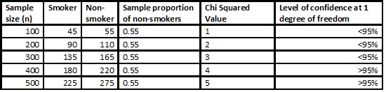
An expert is curious and calculates chi-squared values with the same sample proportion of non-smokers but with increasing sample size as below:

Table 1: Sample size with Same Sample Proportion of Non-Smokers, Chi Squared Value and Level of Significance

An expert finds that upto 300 samples, an expert is less than 95 confident that the sample truly represents the population and there remains high sampling error. As the sample size increase from 400 to more, an expert is more than 95 percent confident and sampling error remains lower. Thus, at least 400 sample size is required for the sample proportion of non-smokers equal to 0.55 to significantly outnumber the sample proportion of smokers (0.45). In other words, 400 respondents need to be sampled for 55 percent non-smokers to significantly outnumber 45 percent smokers.

One Sample Proportion for Statistical Significance and Sample Size, Statistical Note 43

As the sample size increases, even slightly bigger proportion of category of interest could significantly outnumber another category of binary response.

For example, an expert is interested in knowing the proportion of smokers from the randomly selected sampled respondents. An expert assumes that half of adult population are smokers. An expert administers a question to the adults – Are you a smoker? The respondent responds to the two categories response – Yes or No.

An expert estimates that how many non-smokers would statistically outnumber the smokers to draw valid conclusion. An expert uses the following formula to calculate the minimum number of non-smokers from the given sample size to outnumber the smokers:

 z=(p’-p)/√(pq/n)

  where ,

z=Test statistic, standard normal variate, with a value of 1.96 at 95% level of confidence

p’=Sample proportion of non-smokers

p=Population proportion of non-smokers, equal to 0.50

q= Population proportion of smokers, equal to 0.50

n=Sample size

An expert tries with a sample size of 10 individuals and calculates the minimum sample proportion or number of non-smokers required to statistically significant outnumber the smokers. Gradually he increases the sample size and calculates the minimum sample proportion and number of non-smokers required to statistically outnumber the smokers as shown in the table below:

Table 1: Number of Non-Smokers Required to Statistically Significant Outnumber the Smokers

An expert assumes whether six out of 10 non-smokers or the sample non-smoker proportion of 0.60 is enough for statistically significance to outnumber smokers. An expert then used the above formula and finds that the sample non-smoker proportion of 0.8099 or eight non-smokers out of 10 respondents are required for statistically significant outnumber the smokers. Gradually, an expert tries with one hundred thousand hypothetical sample size of respondents with the assumption that 50,001 non-smokers would outnumber 49,999 smokers. Unlike, using the formula an expert finds that the sample non-smoker proportion of 0.5030 or 50,300 non-smokers are required for statistically significant outnumber the smokers. An expert finally understands that as the sample size increases, the smaller sample proportion of non-smokers than the assumed sample proportions presented in the realtime column in the table could significantly outnumber the smokers.