Level of Confidence Increases with Sample Size: An Example of One Sample Proportion, Statistical Note 47

Level of confidence increases with an increase in sample size for one sample proportion. This note tries to exemplify this fact by using the process and data discussed in my statistical note 43 and 44 respectively.

For example, an expert is interested in knowing the proportion of non-smokers from the randomly sampled respondents (following randomization, the first rule of sample proportion). An expert assumes that half of adult population are smokers. An expert administers a question to the randomly adults – Are you a smoker? The respondents answer to one of two categories of response – Yes or No.

An expert tries with a sample size of 100 adults and finds that 55 are non-smokers and remaining 45 are smokers (following normality that non-/smokers need to be at least 10, second rule of sample proportion). An expert then retains the same sample proportion of smokers and hypothetically increases the sample size by 100 to 500. An expert assumes to follow independence in sampling without replacement that the population size is more than 10 times of sample size, third rule of sample proportion.

An expert estimates how confident he is in deciding that non-smokers statistically outnumber the smokers with the increase in sample size. An expert uses the following formula to calculate the minimum number of non-smokers from the given sample size to outnumber the smokers:

 z=(p^-p)/√(pq/n)

  where ,

z=Test statistic, standard normal variate, with a value of 1.96 at 95% level of confidence

p^=Sample proportion of non-smokers

p=Population proportion of non-smokers, equal to 0.50

q= Population proportion of smokers, equal to 0.50

n=Sample size

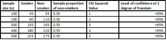
Table 1: Sample size with Same Sample Proportion of Non-Smokers and Level of Confidence to Conclude Non-Smokers Outnumber Smokers

An expert is 84 percent confident in deciding that the sample non-smoker proportion of 0.55 among 100 respondents statistically outnumbers the sample smoker proportion of 0.45. Usual threshold is that decisions are made at 95 percent level of confidence. Gradually, an expert increases sample size by 100 and finds that for a sample of 300 respondents or more an expert is more than 95 percent confident in deciding that the sample proportion of non-smokers equal to 0.55 is statistically higher than the sample proportion of smokers equal to 0.45. It proves that the level of confidence increases as sample size increases for one sample proportion.

Conditional and Joint Probabilities from an Exemplary Survey Dataset, Statistical Note 46

Understanding the concepts of joint and conditional probabilities and developing the skill to apply the concepts to calculate from the given dataset is important in the real time.

An exemplary survey dataset constitutes one hundred records of randomly sampled respondents categorized by smoking habit (smokers or non-smokers) and food habit (vegetarians or non-vegetarians). A part of the dataset in value label view of SPSS is shown in Table 1. Calculate the probability that a randomly sample respondent is a non-smokers is a non-vegetarian.

Table 1: Part of a dataset with smoking and food habits

Concept

Calculating the probability of a "AND" compound event that a randomly selected respondent is a smoker who is a vegetarian also includes calculating the probabilities of other events. Several concepts are introduced while answering this question.

This example has two discrete random variables or categorical variables each with two mutually exclusive categories of response. One categorical variable is the smoking habit of a randomly sampled respondent which has two categories of response: smoker (S) or non-smoker (NS). Another categorical variable is the food habit which also has two mutually exclusive categories: vegetarian (V) and non-vegetarian (NV).

Simple or marginal probability: Let ‘S’ be a random event that a randomly sampled respondent is a smoker. The probability of randomly sampled smoker, represented by P(S) is the total number of smokers divided by total number of respondents. It is also referred to as the relative frequency. Similarly, P(NS), P(V) and P(NV) are calculated.

Conditional probability: Let V/S be a simple event that a participant is a vegetarian among the smokers. The conditional probability of vegetarians among smokers symbolized by P(V/S) is total number of vegetarians among smokers divided by total number of smokers. Here the occurrence of the event of vegetarian smoker is dependent on the event of occurrence of smokers.

Joint Probability: Let ‘S intersection V’,  ‘S∩V’ or ‘S and V’ is a "AND" compound event that a respondent is a smoker and a vegetarian. Here, the multiplication rule of two dependent events is applied. The joint probability of two dependent events is the product of a marginal probability and the conditional probability. In this case, the joint probability of a smoker who is a vegetarian indicated by P(S intersection V), P(S∩V) or P(S and V) in which both events of smoker and vegetarian among all smokers occur is the product of P(S) and P(V/S). Likewise, P(NV/S), P(V/NS), P(NV/NS), P(NS∩V), P(S∩NV) and P(NS∩NV) are calculated.

Calculation

A contingency or cross table from the given survey dataset can be generated either in SPSS or Excel package upon the availability of the software.  In SPSS, using the function ‘Crosstabs’ in Descriptive Statistics’ group of ‘Analyze’ tab, one can get the cross table as in Table 2. In Excel, ‘Pivot Table’ function in the ‘Tables’ group in ‘Insert’ tab can be used to generate cross table like this.

Table 2: Cross table of smoking habit and food habit

Table 2 constituting four cells and totals to presents the frequencies, row percent (% within SMOKE), column percent (% within VEG) and percent of total respondents. Now, the concepts discussed above are applied to calculate probabilities.

Simple or Marginal Probability: Table summarizes that 25 out of 100 respondents are smokers so that P(S) is equal to 0.25, which is 25 percent in percentage term as shown by ‘% of Total’. P(NS) is 0.75 or 75 percent in percentage term. Likewise, P(V) is 0.25 or 25 percent in percentage term and P(NV) is 0.75 or 75 percent in percentage term.

Conditional Probability: P(V/S) is calculated looking at the first cell of the table. Eight out of 25 smokers are vegetarians so that P(V/S) is equal to eight divided by 25 equal to 0.32, which is equal to the row percent (% within SMOKE) of 32% in percentage terms. Similarly, other conditional probabilities are calculated as P(NV/S)=0.68, P(V/NS)=0.227, P(NV/NS)=0.773.

Joint probability: P(S∩V) is the product of P(S) and P(V/S), equal to the product of (25 by 100 ) and (eight by 25), equal to 0.08 or 8 percent in percentage term. This is equal to ‘% of Total’ in the first cell of Table 2.

Upon filling manually the probability values in yellow highlights of Table 2, the table looks as Table 3. The joint probability for each cell is equal to percent of total value in percentage term.

Table 3: Cross table of smoking habit and food habit with probabilities manual added

It is hoped that such a simple example will help create curiosity among the readers as to applying the concept in the real time data.

Simple Probability Calculation from an Exemplary Survey Dataset, Statistical Note 45

Understanding the concept of simple or marginal probability and developing the skill to apply the concept to calculate from the given dataset is important in the real time.

An exemplary survey dataset constitutes one hundred records of randomly sampled respondents categorized as smokers or non-smokers. A part of the dataset in value label view of SPSS is shown in Table 1. Calculate the probability that a randomly sample respondent is a non-smokers.


Table 1: Part of dataset of smokers and non-smokers

Concept 

Simple or marginal probability of an event is the total number of favorable cases divided by total number of cases. Let ‘S’ be a simple event that a participant is a smoker and the simple or the marginal probability of ‘S’ represented by P(S) is the total number of smokers divided by total number of respondents. It is also referred to as the relative frequency.

Calculation 

The survey dataset can be summarized either in SPSS or Excel package upon the availability of the software.  In SPSS, using the function ‘Frequencies’ in Descriptive Statistics’ group of ‘Analyze’ tab, one can get the frequency table as in Table 2.
 

Table 2: Frequency table of smokers and non-smokers

In Excel, ‘Descriptive Statistics’ function in the ‘Data Analysis’ Add-In program can be used to generate frequency table.

The percent or valid percent column shows that 20 percent of respondents are non-smokers. It means that 20 out of 100 respondents are non-smokers.   Thus, the simple or marginal probability that a randomly sampled respondent is a non-smokers is calculated as 20 divided by 100 equal to 0.20. Similarly, the simple or marginal probability of smokers can be calculated to be 0.80.
 I hope this simple example will help create curiosity among the readers as to applying the concept in the real time data.

Same Sample Proportion with Different Sample Sizes for Chi-Squared Test for Goodness of Fit, Statistical Note 44

The level of confidence for statistical significance varies with the variation in the sample size of the same sample proportion.

For example, an expert is interested in knowing the proportion of smokers from the randomly selected sampled respondents. An expert assumes that half of adult population are smokers. An expert administers a question to the adults – Are you a smoker? The respondents respond to one of two categories of response – Yes or No.

An expert tries with a sample size of 100 individuals and finds that 55 respondents are non-smokers and remaining 45 are smokers. He uses Chi-Squared test for goodness of fit to test whether the sample proportions of non-smokers and smokers represent the population proportions, using the formula for one degree of freedom as below:

Chi-square = Sum(O_i-E_i)²/E_i

where:

O_i = Sampled/ observed proportion for _ith category

E_i = population/ expected proportion for _ith category

Using above formula, an expert calculates Chi-squared value for 100 samples as:

Chi-square =Sum(O_i-E_i)²/E_i = (55-50)²/50+(45-50)²/50 = 1

An expert is curious and calculates chi-squared values with the same sample proportion of non-smokers but with increasing sample size as below:

Table 1: Sample size with Same Sample Proportion of Non-Smokers, Chi Squared Value and Level of Significance

An expert finds that upto 300 samples, an expert is less than 95 confident that the sample truly represents the population and there remains high sampling error. As the sample size increase from 400 to more, an expert is more than 95 percent confident and sampling error remains lower. Thus, at least 400 sample size is required for the sample proportion of non-smokers equal to 0.55 to significantly outnumber the sample proportion of smokers (0.45). In other words, 400 respondents need to be sampled for 55 percent non-smokers to significantly outnumber 45 percent smokers.

One Sample Proportion for Statistical Significance and Sample Size, Statistical Note 43

As the sample size increases, even slightly bigger proportion of category of interest could significantly outnumber another category of binary response.

For example, an expert is interested in knowing the proportion of smokers from the randomly selected sampled respondents. An expert assumes that half of adult population are smokers. An expert administers a question to the adults – Are you a smoker? The respondent responds to the two categories response – Yes or No.

An expert estimates that how many non-smokers would statistically outnumber the smokers to draw valid conclusion. An expert uses the following formula to calculate the minimum number of non-smokers from the given sample size to outnumber the smokers:

 z=(p’-p)/√(pq/n)

  where ,

z=Test statistic, standard normal variate, with a value of 1.96 at 95% level of confidence

p’=Sample proportion of non-smokers

p=Population proportion of non-smokers, equal to 0.50

q= Population proportion of smokers, equal to 0.50

n=Sample size

An expert tries with a sample size of 10 individuals and calculates the minimum sample proportion or number of non-smokers required to statistically significant outnumber the smokers. Gradually he increases the sample size and calculates the minimum sample proportion and number of non-smokers required to statistically outnumber the smokers as shown in the table below:

Table 1: Number of Non-Smokers Required to Statistically Significant Outnumber the Smokers

An expert assumes whether six out of 10 non-smokers or the sample non-smoker proportion of 0.60 is enough for statistically significance to outnumber smokers. An expert then used the above formula and finds that the sample non-smoker proportion of 0.8099 or eight non-smokers out of 10 respondents are required for statistically significant outnumber the smokers. Gradually, an expert tries with one hundred thousand hypothetical sample size of respondents with the assumption that 50,001 non-smokers would outnumber 49,999 smokers. Unlike, using the formula an expert finds that the sample non-smoker proportion of 0.5030 or 50,300 non-smokers are required for statistically significant outnumber the smokers. An expert finally understands that as the sample size increases, the smaller sample proportion of non-smokers than the assumed sample proportions presented in the realtime column in the table could significantly outnumber the smokers.

Pets: Part of one’s family

Handling bulls and old cows has been a nuisance for their owners as they are unproductive or less productive and costs more to rear. In such a case, the government should have a system of tagging the cows and bulls so that the owners can be identified if left open in the streets.
The unproductive or less productive cows and bulls can be reared in a group by some people or organisation so that their feeds are not wasted and their by-products can be used. For example, cow urine is considered holy and also medicinal value, so it can be sold to the users. Cow dung can be used to produce biogas and slurry can be sold to the farmers promoting organic farming or using
biodegradable manures. In other way, the unproductive or less productive cows and bulls can be sold
or given to the organisations such as Jatayu Restaurant, a vulture conservation restaurant. Similarly bulls can be castrated and given to rural households for using as drought power in ploughing land. If the government could ensure the quality of cow milk sold in the market, the government
should charge at least one to some rupees per litre of cow milk as tax to collect fund that goes for the
welfare of bulls and old cows.

Basan Shrestha,
Ghattekulo, Kathmandu

http://epaper.thehimalayantimes.com/html5/reader/production/default.aspx?pubname=&pubid=cd7278e2-4150-475f-8abe-305e5ed57783

If I could, then I would..

PEOPLESPEAK

Data analysis is my present area of interest and will remain in future as well. This is an area of my profession and qualification.

In everyday life people either generate data or use them in some form or the other. Collecting data, arranging them in some order and analyzing them to summarize and compare, visualize and use to generate information for reflection and decision making are important actions that data fascinated- people need to do. There is a general practice that lots of data are collected and dumped into the warehouse unused. If there are opportunities to access huge set of data, I would screen them, analyze and bring information out of them.

Basan Shrestha, Ghattekulo, Kathmandu

http://epaper.thehimalayantimes.com/html5/reader/production/default.aspx?pubname=&pubid=cd7278e2-4150-475f-8abe-305e5ed57783

Multiplication Rule of Mutually Exclusive and Inclusive Events, Statistical Note 42

Mutually Exclusive Events: Two events are mutually exclusive if they cannot occur at the same time. In tossing of a coin, either of head or tail flips meaning they are mutually exclusive. An occurrence of head excludes an occurrence of tail in the same toss.

Let H be an event of turning head in a toss of a coin.  Likewise, let T be an event of turning tail in a toss of a coin.  The marginal probability of H, P(H) is one by two, 0.5. Similarly, the marginal probability of T, P(T) is one by two, 0.5. The joint probability of head and tail in a single toss, denoted by P(H and T) is impossible, equal to zero.

Figure 1: Marginal probabilities in tossing of a coin

Likewise, in drawing a card from the deck of 52 cards, the occurrence of an ace card excludes cards of other ranks, two to ten, jack, queen and king. Let A be an event of drawing an ace card.  Likewise, let B be an event of drawing any non-ace card.  The marginal probability of A, P(A) is four by 52 or one by 13. Similarly, the marginal probability of any non-ace card, P(B) is 48 by 52 or 12 by 13. The joint probability of ace and any non-ace card in a single draw, denoted by P(A and B) is impossible, equal to zero.

Figure 2: Marginal probabilities in drawing a card from a deck

Mutually Inclusive Events: Two events are mutually inclusive or non-exclusive if the occur of an event does not exclude the occurrence of another event at the same time. In drawing a card from the deck of 52 cards, the occurrence of an ace card does not exclude the occurrence of a club card. Because, both identities - ace as a rank and club as a suit exist on the same card.

Let A be an event of drawing an ace card.  Likewise, let B be an event of drawing any non-ace card.  The marginal probability of A, P(A) is four by 52 or one by 13. Similarly, the marginal probability of any non-ace card, P(NA) is 48 by 52 or 12 by 13. Likewise, let C be an event of drawing a club card and NC be an event of drawing a non-club card. The joint probability of ace and club card in a single draw, denoted by P(A and C) is the product of P(A) and P(C), equal to 0.0192. Similarly, P(A and NC), P(NA and C) and P(NA and NC) are equal to 0.056, 0.2307 and 0.6923 respectively as shown in Figure 3.

Figure 3: Marginal probabilities of mutually exclusive events and joint probability of mutually inclusive events in a draw of a card from the deck

Mutually Exclusive and Inclusive Events: Examples, Statistical Note 41

Mutually Exclusive Events: Two events are mutually exclusive if they cannot occur at the same time. In tossing of a coin, either of head or tail flips meaning they are mutually exclusive. An occurrence of head excludes an occurrence of tail in the same toss. 

In another example of drawing a card from the deck of 52 cards, the occurrence of an ace card excludes cards of other ranks, two to ten, jack, queen and king.

Mutually Inclusive Events: Two events are mutually inclusive or non-exclusive if the occur of an event does not exclude the occurrence of another event at the same time. In drawing a card from the deck of 52 cards, the occurrence of an ace card does not exclude the occurrence of a club card. Because, both identities - ace as a rank and club as a suit exist on the same card.

Heads and Runs in Multiple Tossing of a Coin and Contingency Table, Statistical Note 40

List the possible outcomes in three tosses of a coin, categorize them by the number of number of heads and the number of runs in the sequence and prepare a contingency table.

Tossing of a coin thrice has two to the power three equal to eight possible outcomes (refer to my statistical note 9). Every outcome is measured using two discrete random variables – the number of heads and the number of runs. The outcomes have number of heads ranging from zero to three as mutually exclusive categories of response as shown in Table 1. A run is a sequence of flips of the same face of a coin. The number of runs ranges from one to three as mutually exclusive categories of response (Table 1). Example, an outcome HTH has three runs, as every toss has a different face than the previous toss. A contingency table, also known as the cross tabulation, crosstab or two-way table counts the number observations for each category of two variables.

Table 1: Possible outcomes in three tosses of a coin by number of heads and number of runs

The contingency table presents the number of possible outcomes by number of heads and number of runs (Table 2).

Central values of both variables have high probability of occurrence. Example, outcomes with one and two heads respectively have higher probability of occurrence, three by eight. Likewise, outcomes with two runs have higher probability of occurrence, four by eight. Refer to my statistical note 3 for probability and contingency table.

Multiplication Rule of Dependent Events, Statistical Note 39

If two cards are drawn without replacement from a deck of cards, what is the joint probability that both cards are red?

The multiplication rule of probability of two dependent events is the product of the probability of first independent marginal event and the conditional probability of second dependent marginal event. Same applies to the joint probability of multiple dependent events.

Symbolically, let A be an independent event and B be a dependent event, the joint probability that both events and A and B occur is stated as:

P(A and B) = P(A)*P (B/A), where P(A) is the probability of an independent event A and P(B/A) is the conditional probability of a dependent event B given the occurrence of an independent event A.

The events are said to be dependent events if the occurrence of the first event affects the probability of the second and following events. In this example, drawing of a red card in the first event and not replacing back that card to the deck of cards before second draw of a card affects the second draw of a card. This applies to multiple draws of cards without replacement from a deck of cards.

Let R1 be an independent event of drawing a red card in the first draw of a card.  There are 26 red cards in a deck of cards. The marginal probability of R1, P(R1) is 26 divided by 52, 0.5. Let R2 be a dependent event of drawing a red card from the deck of cards in which the first drawn card is not replaced back.  There are 25 red cards left in the deck of 51 cards, as the first drawn cards is red which is not replaced back in the deck. Thus, the conditional probability of R2 given R1 in the first draw, P(R2/R1) is 25 divided by 51, 0.4902.

Now, applying the multiplication rule of dependent events, the joint probability that red cards are drawn in both draws without replacement is the product of P(R1) in the first draw and the P(R2) in the second draw.

Symbolically, P(R1 and R2) = P(R1)*P (R2/R1)=26/52 *25/51 =0.2450

The total number of outcomes in two draws of cards without replacement from a deck of cards and their probabilities are shown using a tree diagram below:

Figure 1: Marginal probabilities of first draws and conditional probabilities of second draws given the first draws of cards without replacement and joint probabilities of possible outcomes

Time to Break Gender Stereotype of All Kinds

There could be gender stereotypes in some professions in the past leading people to perceive a man is a doctor and a woman a nurse, a man is a pilot and a woman an airhostess. However, there is nothing that men can do and women cannot or vice versa in this millennium. The constitution clearly prohibits against discriminating on the grounds of gender in remuneration and social security for the same work. A male doctor can be a gynecologist and a female doctor can treat a male reproductive organ.  Equal opportunity for men and women needs to be given in every profession. Thus, gender stereotypes need to be discouraged by creating awareness, creating opportunities and taking legal actions against the violation of the rules.

Basan Shrestha, Ghattekulo, Kathmandu

The Himalayan Times, PeopleSpeak, May 12, 2019

http://epaper.thehimalayantimes.com/html5/reader/production/default.aspx?pubname=&pubid=cd7278e2-4150-475f-8abe-305e5ed57783

Multiplication Rule of Independent Events, Statistical Note 38

If an unbiased coin with two sides (Head and Tail) is tossed twice, what is the joint probability that head appears in both tosses?

The multiplication rule of probability of two independent events is the product of the probability of first independent marginal event and the probability of second independent marginal event. Same applies to the joint probability of multiple independent events.

Symbolically, if two events A and B are independent, the probability that both events and A and B occur is stated as:

P(A and B) = P(A)*P (B)

The events are said to be independent events if the occurrence of the first event does not affect the probability of the second and following events. In this example, occurrence of head or tail in the first toss does not affect the occurrence of head or tail in the second toss. Any of head or tail could appear in any number of toss of a coin. This applies to multiple tosses of a coin.

Let H be an independent event of turning head in a toss of a coin.  Likewise, let T be an independent event of turning tail in a toss of a coin.  The marginal probability of H, P(H) is one by two, 0.5. Similarly, the marginal probability of T, P(T) is one by two, 0.5.

The total number of outcomes in two tosses of a coin can be shown a tree diagram like the one shown below:

Figure 1: Marginal probabilities of independent events in first and second tosses of a coin and number of outcomes

Now, applying the multiplication rule of independent events, the joint probability that head appears in both tosses is the product of P(H) in the first toss and the P(H) in the second toss.

Symbolically, P(H and H) = ½ * ½ = ¼ = 0.25

Alternatively, the occurrence of head in both tosses is Outcome 1 of four outcomes in the tree diagram, and thus the probability is one out of four, equal to 0.25.